
1. bike 데이터셋
import numpy as np
import pandas as pd
import matplotlib.pyplot as plt
import seaborn as sns

bike_df = pd.read_csv('/content/drive/MyDrive/KDT v2/머신러닝과 딥러닝/ data/bike.csv')
bike_df.info()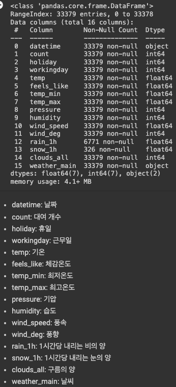
sns.displot(bike_df['count'])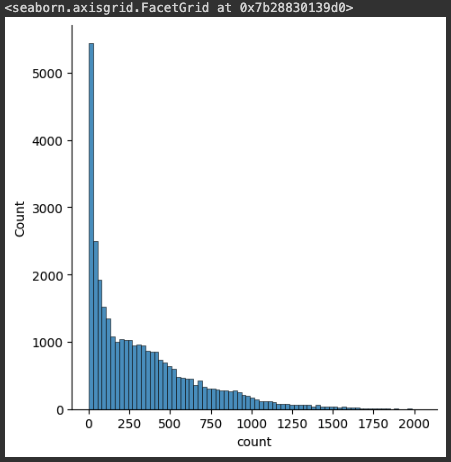
sns.boxplot(y=bike_df['count'])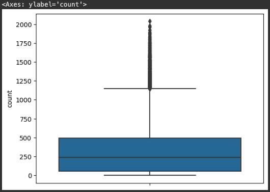
sns.scatterplot(x='feels_like', y='count', data=bike_df, alpha=0.3)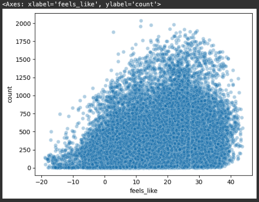
sns.scatterplot(x='pressure', y='count', data=bike_df, alpha=0.3)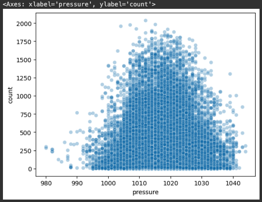
sns.scatterplot(x='wind_speed', y='count', data=bike_df, alpha=0.3)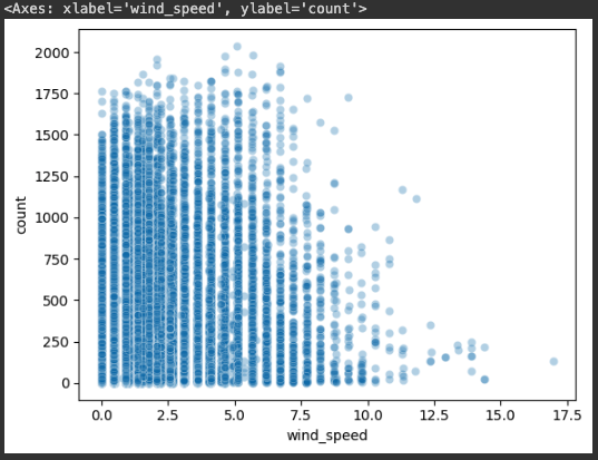
sns.scatterplot(x='wind_deg', y='count', data=bike_df, alpha=0.3)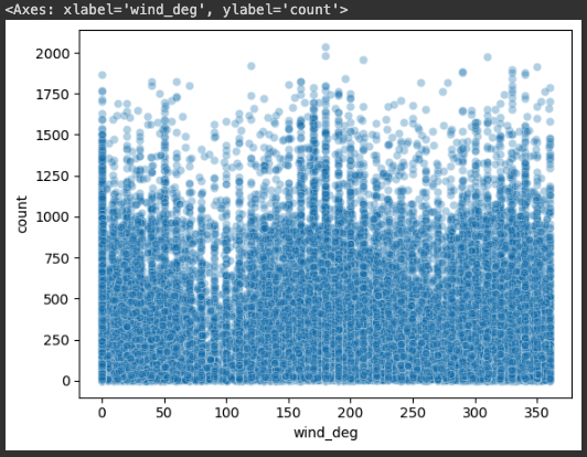
bike_df.isna().sum()
# 결과값 =>
# datetime            0
# count               0
# holiday             0
# workingday          0
# temp                0
# feels_like          0
# temp_min            0
# temp_max            0
# pressure            0
# humidity            0
# wind_speed          0
# wind_deg            0
# rain_1h         26608
# snow_1h         33053
# clouds_all          0
# weather_main        0
# dtype: int64
bike_df=bike_df.fillna(0)
bike_df['datetime'] = pd.to_datetime(bike_df['datetime'])
bike_df.info()
# 결과값 =>

# <class 'pandas.core.frame.DataFrame'>
# RangeIndex: 33379 entries, 0 to 33378
# Data columns (total 16 columns):
#  #   Column        Non-Null Count  Dtype
# ---  ------        --------------  -----
#  0   datetime      33379 non-null  datetime64[ns]
#  1   count         33379 non-null  int64
#  2   holiday       33379 non-null  int64
#  3   workingday    33379 non-null  int64
#  4   temp          33379 non-null  float64
#  5   feels_like    33379 non-null  float64
#  6   temp_min      33379 non-null  float64
#  7   temp_max      33379 non-null  float64
#  8   pressure      33379 non-null  int64
#  9   humidity      33379 non-null  int64
#  10  wind_speed    33379 non-null  float64
#  11  wind_deg      33379 non-null  int64
#  12  rain_1h       33379 non-null  float64
#  13  snow_1h       33379 non-null  float64
#  14  clouds_all    33379 non-null  int64
#  15  weather_main  33379 non-null  object
# dtypes: datetime64[ns](1), float64(7), int64(7), object(1)
# memory usage: 4.1+ MB
bike_df['year'] = bike_df['datetime'].dt.year
bike_df['month'] = bike_df['datetime'].dt.month
bike_df['hour'] = bike_df['datetime'].dt.hour
bike_df['date'] = bike_df['datetime'].dt.date
plt.figure(figsize=(14, 4))
sns.lineplot(x='date', y='count', data=bike_df)
plt.xticks(rotation=45)
plt.show()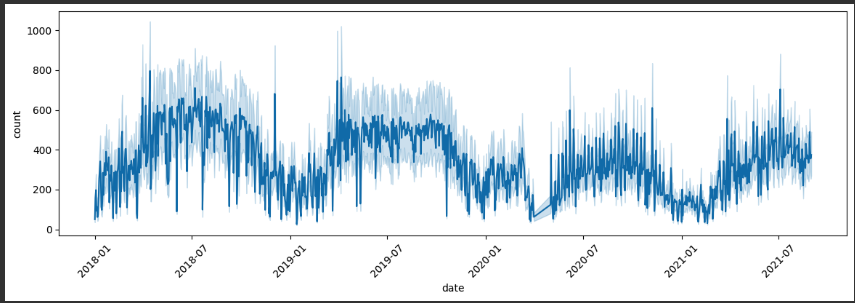
bike_df[bike_df['year'] == 2019].groupby('month')['count'].mean()
# 결과값 =>
# month
# 1     193.368862
# 2     221.857718
# 3     326.564456
# 4     482.931694
# 5     438.027848
# 6     478.480053
# 7     472.745785
# 8     481.267366
# 9     500.862069
# 10    446.279070
# 11    307.295393
# 12    213.148886
# Name: count, dtype: float64
bike_df[bike_df['year'] == 2020].groupby('month')['count'].mean()
# 결과값 =>
# month
# 1     260.445997
# 2     255.894320
# 3     217.135241
# 5     196.581064
# 6     290.900937
# 7     299.811688
# 8     331.528809
# 9     338.876478
# 10    293.640777
# 11    240.507324
# 12    138.993540
# Name: count, dtype: float64
# covid
# 2020-04-01 이전: precovid
# 2020-04-01 이후 ~ 2021-04-01 이전 : covid
# 2021-04-01 이후 : postcovid
def covid(date):
    if str(date) < '2020-04-01':
        return 'precovid'
    elif str(date) < '2021-04-01':
        return 'covid'
    else :
        return 'postcovid'
bike_df['date'].apply(covid)
# 결과값 =>
# 0 precovid
# 1 precovid
# 2 precovid
# 3 precovid
# 4 precovid
# ...
# 33374 postcovid
# 33375 postcovid
# 33376 postcovid
# 33377 postcovid
# 33378 postcovid
# Name: date, Length: 33379, dtype: object
bike_df['covid'] = bike_df['date'].apply(lambda date: 'precovid' if str(date) < '2020-04-01' else 'covid' if str(date) < '2021-04-01' else 'postcovid')
# season
# 12월 ~ 2월: winter
# 3월 ~ 5월 : spring
# 6월 ~ 8월 : summer
# 9월 ~ 11월 : fall

bike_df['season'] = bike_df['month'].apply(lambda x: 'winter' if x == 12 else 'fall' if x >= 9 else 'summer' if x >= 6 else 'spring' if x >= 3 else 'winter')
bike_df[['month', 'season']]
# day_night
# 21 이후 ~ : night
# 19 이후 ~ : late evening
# 17 이후 ~ : early evening
# 16 이후 ~ : late afternoon
# 13 이후 ~ : early afternoon
# 11 이후 ~ : late morning
# 05 이후 ~ : early morning

bike_df['day_night'] = bike_df['hour'].apply(lambda x: 'night' if x >= 21
                                             else 'late evening' if x >= 19
                                             else 'early evening' if x>= 17
                                             else 'late afternoon' if x>= 16
                                             else 'early afternoon' if x>= 13
                                             else 'late morning' if x>= 11
                                             else 'early morning' if x>= 5
                                             else 'night')
bike_df.drop(['datetime', 'month', 'date', 'hour'], axis=1, inplace=True)
for i in ['weather_main', 'covid', 'season', 'day_night'] :
    print(i, bike_df[i].nunique())

# 결과값 =>
# weather_main 11
# covid 3
# season 4
# day_night 7
bike_df['weather_main'].unique()
# 결과값 => array(['Clouds', 'Clear', 'Snow', 'Mist', 'Rain', 'Fog', 'Drizzle', 'Haze', 'Thunderstorm', 'Smoke', 'Squall'], dtype=object)
bike_df = pd.get_dummies(bike_df, columns=['weather_main', 'covid', 'season', 'day_night'])
from sklearn.model_selection import train_test_split
X_train, X_test, y_train, y_test = train_test_split(bike_df.drop('count', axis=1), bike_df['count'], test_size=0.2, random_state=2023)
2. 의사 결정 나무(Decision Tree)
- 데이터를 분석하고 패턴을 파악하여 결정 규칙을 나무 구조로 나타낸 기계학습 알고리즘
- 간단하고 강력한 모델 중 하나로, 분류와 회귀 문제 모두 사용가능
- 지니계수(지니 불순도, Gini Impurity) : 분류 문제에서 특정 노드의 불순도를 나타내는데, 노드가 포함하는 클래스들이 혼잡되어 있는 정도를 나타냄
- 0에서 1개까지의 값을 가지며, 0에 가까울 수록 노드의 값이 불순도가 없음을 의미
- 로그 연산이 없어 계산이 상대적으로 빠름
- 엔트로피 : 어떤 집합이나 데이터의 불확실성, 혼잡도를 나타내는데, 노드의 불순도를 측정하는데 활용
- 0에서 무한대까지의 값을 가지며, 0에 가까울수록 노드의 값이 불순도가 없음을 의미
- 로그 연산이 포함되어 있어 계산이 복잡
- 오버피팅(과적합) : 학습데이터에서는 정확하나 테스트데이터에서는 성과가 나쁜 현상을 말함. 의사 결정 나무는 오버피팅이 매우 잘 일어남
- 오버피팅을 방지하는 방법
- 사전 가지치기 : 나무가 다 자라기 전에 알고리즘을 멈추는 방법
- 사후 가지치기 : 나무를 끝까지 돌린 후 밑에서 부터 가지를 쳐나가는 방법
- 오버피팅을 방지하는 방법
from sklearn.tree import DecisionTreeRegressor # 예측
dtr = DecisionTreeRegressor(random_state=2023)
dtr.fit(X_train, y_train)
pred1 = dtr.predict(X_test)
sns.scatterplot(x=y_test, y=pred1)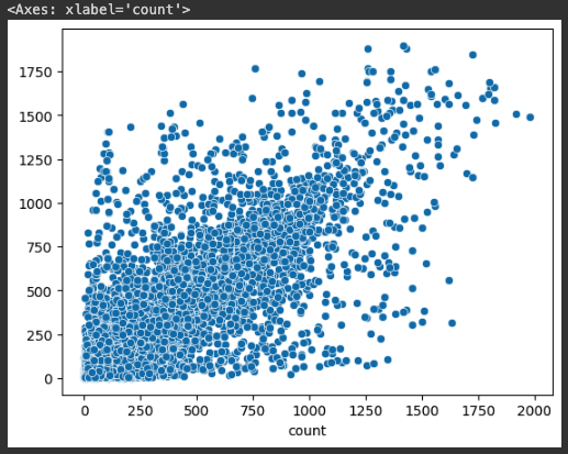
from sklearn.metrics import mean_squared_error # 오차값 측정
mean_squared_error(y_test, pred1, squared=False)
# 결과값 => 222.90547303762153
3. 선형 회귀 vs 의사 결정 나무
from sklearn.linear_model import LinearRegression
lr = LinearRegression()
lr. fit(X_train, y_train)
pred2 = lr.predict(X_test)
sns.scatterplot(x=y_test, y=pred2)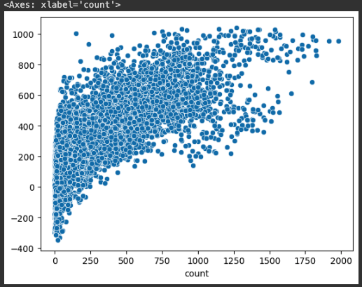
mean_squared_error(y_test, pred2, squared=False)
# 결과값 => 224.5257704711731

# 의사 결정 나무 : 222.90547303762153
# 선형 회귀 : 224.5257704711731
222.90547303762153 - 224.5257704711731
# 결과값 => -1.6202974335515705
# 하이퍼 파라미터 적용
dt = DecisionTreeRegressor(random_state=2023, max_depth=50, min_samples_leaf=30)
# max_depth는 사전 가지치기 50덱스까지만 내려가라.
# min_sample_leaf = 최소 셈플의 잎파리 수가 30개는 되어야한다.

dt.fit(X_train, y_train)
pred3 = dt.predict(X_test)
mean_squared_error(y_test, pred3, squared=False)
# 결과값 => 186.56448037541028

# 의사 결정 나무 : 222.90547303762153
# 의사 결정 나무(하이퍼 파라미터 튜닝) : 186.56448037541028
186.56448037541028 - 222.90547303762153
# 결과값 => -36.34099266221125
from sklearn.tree import plot_tree
# 인덱스를 이용해서 뽑는 기준. X38번째 컬럼을 찾아라 근데 찾기 귀찮으니 아래는 컬럼명을 출력해서 보여줌
plt.figure(figsize=(24, 12))
plot_tree(dtr, max_depth=5, fontsize=12)
plt.show()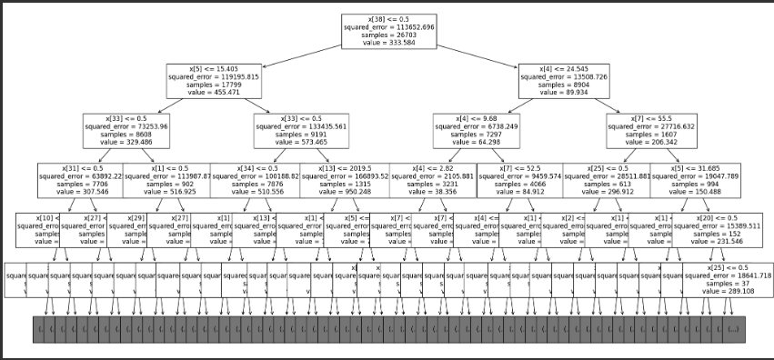
# 컬럼명을 이용해서 출력
plt.figure(figsize=(24, 12))
plot_tree(dtr, max_depth=5, fontsize=12, feature_names=X_train.columns)
plt.show()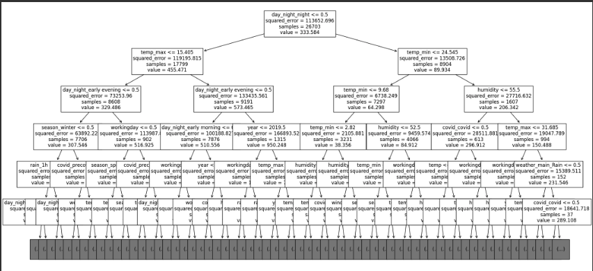
'Study > 머신러닝과 딥러닝' 카테고리의 다른 글
| [머신러닝과 딥러닝] 8. 서포트 백터 머신 (0) | 2024.01.02 |
|---|---|
| [머신러닝과 딥러닝] 7. 로지스틱 회귀 (0) | 2024.01.02 |
| [머신러닝과 딥러닝] 5. 선형 회귀 (0) | 2023.12.28 |
| [머신러닝과 딥러닝] 4. 타이타닉 데이터셋 (0) | 2023.12.27 |
| [머신러닝과 딥러닝] 3. 아이리스 데이터셋 (0) | 2023.12.23 |