
1. Cluster(클러스터)
- 유사한 특성을 가진 객체들의 집합
- 고객 분류, 유전자 분석, 이미지 분할
import numpy as np
import pandas as pd
import seaborn as sns
import matplotlib.pyplot as plt
from sklearn.datasets import make_blobs

# X는 2차원으로 된 데이터 프레임
# y는 데이터 답을 만들어줌
X, y = make_blobs(n_samples=100, centers=3, random_state=10)
# n_samples = 샘플을 몇개를 만들지
# centers = 몇가지의 클래스를 만들지, 군집데이터를 만들기 때문에 class가 아닌 centers라고 작성함
X

# 결과값 =>
# array([[ -2.32496308,  -6.6999964 ],
#        [  0.51856831,  -4.90086804],
#
#        ...
#
#        [  5.40050753,  -9.29586681]])
X = pd.DataFrame(X) # 데이터 프레임으로 변환
X
y

# 결과값 =>
# array([2, 2, 1, 0, 1, 1, 0, 2, 1, 0, 0, 1, 1, 2, 2, 1, 0, 1, 0, 1, 0, 2,
#        1, 2, 0, 1, 1, 1, 1, 0, 2, 1, 1, 0, 2, 2, 2, 1, 1, 1, 2, 0, 2, 2,
#        1, 0, 0, 0, 2, 0, 1, 2, 0, 0, 2, 0, 1, 2, 0, 0, 1, 1, 2, 2, 2, 0,
#        0, 2, 2, 2, 1, 0, 1, 1, 2, 1, 1, 2, 0, 0, 0, 1, 0, 1, 2, 1, 2, 0,
#        2, 2, 0, 0, 0, 2, 2, 2, 1, 0, 0, 0])
sns.scatterplot(x=X[0], y=X[1], hue=y)
from sklearn.cluster import KMeans

km = KMeans(n_clusters=3)
# 학습
km.fit(X)
# 예측
pred = km.predict(X)

sns.scatterplot(x=X[0], y=X[1], hue=pred)
km = KMeans(n_clusters=5)
# 학습
km.fit(X)
# 예측
pred = km.predict(X)

sns.scatterplot(x=X[0], y=X[1], hue=pred)
# 평가값 : 하나의 클러스트안에 중심점으로부터 각각의 데이터 거리를 합한 값의 평균
km.inertia_
# 값이 크면 데이터간 거리가 멀어 다른 데이터와 붙어있을가능성이 높음
# 값이 낮으면 데이터가 서로 옹기종기 모여있어 집합이 잘 되어있다

# 결과값 => 130.02425208172426

inertia_list = []

for i in range(2, 11) :
    km = KMeans(n_clusters=i)
    km.fit(X)
    inertia_list.append(km.inertia_)

inertia_list

# 결과값 =>
# [976.8773336900748,
#  186.3658862010144,
#  154.03820014871644,
#  130.61963601864812,
#  113.17852746430522,
#  98.39597533978201,
#  84.97468994763855,
#  73.1518886343043,
#  65.03279448102089]
# 엘보우 메서드
sns.lineplot(x=range(2, 11), y=inertia_list)
# 당연히 쪼갤 수록 값이 떨어지는게 당연하면서
# 가장 최적의 값은 심하게 꺽이는 부분이 가장 깔끔하면서 최적화된 부분이라고 판단하면 된다.
2. Marketing 데이터셋
mkt_df = pd.read_csv('/content/drive/MyDrive/KDT v2/머신러닝과 딥러닝/ data/marketing.csv')
mkt_df
mkt_df.info()

# 결과값 =>
#  #   Column               Non-Null Count  Dtype
# ---  ------               --------------  -----
#  0   ID                   2240 non-null   int64
#  1   Year_Birth           2240 non-null   int64
#  2   Education            2240 non-null   object
#  3   Marital_Status       2240 non-null   object
#  4   Income               2216 non-null   float64
#  5   Kidhome              2240 non-null   int64
#  6   Teenhome             2240 non-null   int64
#  7   Dt_Customer          2240 non-null   object
#  8   Recency              2240 non-null   int64
#  9   MntWines             2240 non-null   int64
#  10  MntFruits            2240 non-null   int64
#  11  MntMeatProducts      2240 non-null   int64
#  12  MntFishProducts      2240 non-null   int64
#  13  MntSweetProducts     2240 non-null   int64
#  14  MntGoldProds         2240 non-null   int64
#  15  NumDealsPurchases    2240 non-null   int64
#  16  NumWebPurchases      2240 non-null   int64
#  17  NumCatalogPurchases  2240 non-null   int64
#  18  NumStorePurchases    2240 non-null   int64
#  19  NumWebVisitsMonth    2240 non-null   int64
#  20  Complain             2240 non-null   int64
Customer Data Table
| (영어) | (한글) |
|---|---|
| ID | 고객 아이디 |
| Year_Birth | 출생 연도 |
| Education | 학력 |
| Marital_Status | 결혼 여부 |
| Income | 소득 |
| Kidhome | 어린이 수 |
| Teenhome | 청소년 수 |
| Dt_Customer | 고객 등록일 |
| Recency | 마지막 구매일로부터 경과일 |
| MntWines | 와인 구매액 |
| MntFruits | 과일 구매액 |
| MntMeatProducts | 육류 제품 구매액 |
| MntFishProducts | 어류 제품 구매액 |
| MntSweetProducts | 단맛 제품 구매액 |
| MntGoldProds | 골드 제품 구매액 |
| NumDealsPurchases | 할인 행사 구매 수 |
| NumWebPurchases | 웹에서의 구매 수 |
| NumCatalogPurchases | 카탈로그에서의 구매 수 |
| NumStorePurchases | 매장에서의 구매 수 |
| NumWebVisitsMonth | 월별 웹 방문 수 |
| Complain | 불만 여부 |
mkt_df.isna().sum()

# 결과값 =>
# ID                      0
# Year_Birth              0
# Education               0
# Marital_Status          0
# Income                 24
# Kidhome                 0
# Teenhome                0
# Dt_Customer             0
# Recency                 0
# MntWines                0
# MntFruits               0
# MntMeatProducts         0
# MntFishProducts         0
# MntSweetProducts        0
# MntGoldProds            0
# NumDealsPurchases       0
# NumWebPurchases         0
# NumCatalogPurchases     0
# NumStorePurchases       0
# NumWebVisitsMonth       0
# Complain                0
mkt_df.drop('ID', axis=1, inplace=True)

mkt_df.describe()
mkt_df.sort_values('Year_Birth')
# 내림 차순
mkt_df.sort_values('Income', ascending=False)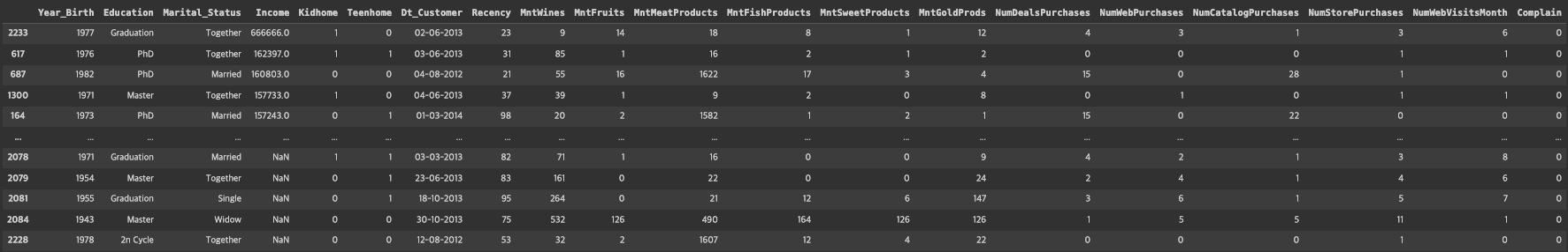
# NaN이 있을때 NaN이 저장되지 않으므로 아래의 코드는 사용 조심.
mkt_df = mkt_df[mkt_df['Income'] != 666666]

mkt_df.sort_values('Income', ascending=False)
# marital_status = widow > 즉 사별(배우자가 사망 혹은 재혼하지 않은 사람)
mkt_df = mkt_df.dropna()

# Dt_Customer : 고겍 등록일
mkt_df['Dt_Customer'] = pd.to_datetime(mkt_df['Dt_Customer'])

# 마지막으로 가입된 사람을 기준으로 현재 데이터의 가입 날짜(달) 차 구하기
# pass_month
mkt_df['pass_month'] = (mkt_df['Dt_Customer'].max().year * 12 + mkt_df['Dt_Customer'].max().month) - (mkt_df['Dt_Customer'].dt.year * 12 + mkt_df['Dt_Customer'].dt.month)
mkt_df.head()

mkt_df.drop('Dt_Customer', axis=1, inplace=True)
# 와인 + 과일 + 육류제품 + 어류 제품 + 단맛 제품 + 골드 제품의 합계 구하기

mkt_df['Total_mnt'] = mkt_df[['MntWines', 'MntFruits', 'MntMeatProducts', 'MntFishProducts', 'MntSweetProducts', 'MntGoldProds']].sum(axis=1)

mkt_df['Children'] = mkt_df[['Kidhome', 'Teenhome']].sum(axis=1)

mkt_df.drop(['Kidhome', 'Teenhome'], axis=1, inplace=True)
mkt_df['Education'].value_counts()
# 결과값 =>
# Graduation    1115
# PhD            481
# Master         365
# 2n Cycle       200
# Basic           54

mkt_df['Marital_Status'].value_counts()
# Married     857
# Together    572
# Single      471
# Divorced    232
# Widow        76
# Alone         3
# Absurd        2
# YOLO          2
mkt_df['Marital_Status'] = mkt_df['Marital_Status'].replace({
    'Married': 'Partner',
    'Together': 'Partner',
    'Single': 'Single',
    'Divorced': 'Single',
    'Widow': 'Single',
    'Alone': 'Single',
    'Absurd': 'Single',
    'YOLO': 'Single',
})

mkt_df['Marital_Status'].value_counts()
# 결과값 =>
# Partner    1429
# Single      786
mkt_df = pd.get_dummies(mkt_df, columns=['Education', 'Marital_Status'])
from sklearn.preprocessing import StandardScaler
ss = StandardScaler()
ss.fit_transform(mkt_df)
pd.DataFrame(ss.fit_transform(mkt_df))
ss_df = pd.DataFrame(ss.fit_transform(mkt_df), columns=mkt_df.columns)
3. KMeans
- K개의 중심점을 찍은 후에, 이 중심점에서 각 점간의 거리의 합이 가장 최소가 되는 중심점 k의 위치를 찾고, 이 중심점에서 가까운 점들을 중심점을 기준으로 묶는 알고리즘
- K개의 클러스터의 수는 정해줘야함
inertia_list = []

for i in range(2, 11) :
    km = KMeans(n_clusters=i, random_state=2024)
    km.fit(ss_df)
    inertia_list.append(km.inertia_)
inertia_list
# 결과값 =>
# [42898.75475762481,
# 39825.85332911935,
# 37620.72546383063,
# 36296.39316484985,
# 34242.24326674706,
# 32502.627684050876,
# 30781.8055617468,
# 29990.604680739903,
# 28248.19018930947]sns.lineplot(x=range(2,11), y=inertia_list)
4. 실루엣 스코어(Silhouette Score)
- 각 군집 간의 거리가 얼마나 효율적으로 분리 되어있는지를 나타냄
- 실루엣 분석은 실루엣 계수를 기반으로 하는데, 실루엣 계수는 개별 데이터가 가지는 군집화 지표
from sklearn.metrics import silhouette_score

score = []

for i in range(2, 11) :
    km = KMeans(n_clusters=i, random_state=2024)
    km.fit(ss_df)
    pred = km. predict(ss_df)
    score.append(silhouette_score(ss_df, pred))
socre
# 결과값 =>
# [0.23022720420084983,
# 0.1422826246539863,
# 0.11964043510714399,
# 0.1281132041299626,
# 0.12161756074874215,
# 0.1252612275778885,
# 0.14543070406681055,
# 0.13864397879387974,
# 0.14911484181076592]sns.lineplot(x=range(2, 11), y=score)
# k의 군집 위치를 찾는건 떨어지는것이 찾는게 아니라 상승폭의 숫자를 보는것이 정답이다. 즉 8이 가장 좋다.
km = KMeans(n_clusters=8, random_state=2024)
km.fit(ss_df)
pred = km.predict(ss_df)
pred
# 결과값 => array([5, 3, 2, ..., 5, 2, 0], dtype=int32)
mkt_df['label'] = pred
# 자기지도학습
mkt_df['label'].value_counts()

# 결과값 =>
# 5    518
# 4    449
# 2    409
# 0    265
# 3    260
# 1    239
# 6     54
# 7 21'Study > 머신러닝과 딥러닝' 카테고리의 다른 글
| [머신러닝과 딥러닝] 14. 파이토치로 구현한 선형회귀_1 (0) | 2024.01.09 |
|---|---|
| [머신러닝과 딥러닝] 13. 파이토치(Pytorch) (1) | 2024.01.09 |
| [머신러닝과 딥러닝] 11. 다양한 모델 적용 (0) | 2024.01.08 |
| [머신러닝과 딥러닝] 10. lightGBM (0) | 2024.01.05 |
| [머신러닝과 딥러닝] 9. 랜덤 포레스트 (0) | 2024.01.03 |